When SQL Server developers begin working with PostgreSQL, indexing usually feels familiar at first. B-tree indexes behave as expected, query plans look readable, and the query planner makes reasonable choices.

But PostgreSQL also introduces new index types like GiST and SP-GiST. They do not map cleanly to anything in SQL Server, and documentation often describes them in abstract terms like “generalized search trees” or “space partitioning”. In this blog posting I try to explain why these index types are necessary, how to think about them coming from SQL Server, and how they work in practice using concrete, reproducible examples.

Why PostgreSQL Needs GiST and SP-GiST

In SQL Server, almost all indexing strategies are based on one central question:

Can this data be ordered in a way that makes the predicate efficient?

If the answer is yes, a B-tree index works. If the answer is no, developers usually fall back to:

• Complex Predicates
• Computed Columns
• or accepting Index Scans

But PostgreSQL takes here a different approach. Instead of forcing all data into linear order, it allows indexes to understand relationships such as overlap, containment, proximity, hierarchy, and prefixes. This is where GiST and SP-GiST come in.

• GiST: temporal and spatial problems where overlap matters
• SP-GiST: hierarchical or prefix-based problems where overlap does not exist

GiST in Practice: Overlapping Time Ranges

Time-based logic is a perfect example of why GiST indexes exists. Bookings, reservations, validity periods, and schedules almost always overlap, and overlap is something a B-tree index cannot model.

PostgreSQL provides native range types, including tsrange (timestamp range). Instead of modeling time periods using two columns, a range is stored as a single value:

TSRANGE(
  '2026-01-10 09:00',
  '2026-01-10 10:30'
)

This represents a period from 09:00 (inclusive) to 10:30 (exclusive) and is internally stored as:

["2026-01-10 09:00:00","2026-01-10 10:30:00")

For SQL Server developers, this replaces the familiar pattern

StartTime DATETIME2,
EndTime   DATETIME2

with a single semantic value.

Let’s have a look on a concrete example. The following code creates a table, and inserts some test data into it:

-- Create a simple table
CREATE TABLE Reservations
(
    ID      BIGINT GENERATED ALWAYS AS IDENTITY PRIMARY KEY,
    RoomID  INT,
    Booking TSRANGE
);

-- Insert some test data
INSERT INTO Reservations (RoomID, Booking) VALUES
(1, tsrange('2026-01-10 08:00', '2026-01-10 10:00')),
(1, tsrange('2026-01-10 09:30', '2026-01-10 11:00')),
(1, tsrange('2026-01-10 11:00', '2026-01-10 12:00')),
(2, tsrange('2026-01-10 09:00', '2026-01-10 10:00'));

-- Additional test data to make the table larger
WITH s AS (
  SELECT
    (random() * 50)::int + 1 AS room_id,
    (timestamp '2026-01-01'
      + (random() * 30) * interval '1 day'
      + (random() * 24) * interval '1 hour'
      + (random() * 60) * interval '1 minute') AS start_ts,
    ((15 + floor(random() * 226))::int * interval '1 minute') AS dur
  FROM generate_series(1, 200000)
)
INSERT INTO Reservations (RoomID, Booking)
SELECT room_id, tsrange(start_ts, start_ts + dur, '[)')
FROM s;

-- Update Statistics
ANALYZE Reservations;

The && Operator: Overlap as a First-Class Concept

The operator && means “overlaps with”. Two ranges overlap if they share at least one point in time.

SELECT *
FROM Reservations
WHERE Booking && TSRANGE(
    '2026-01-10 09:00',
    '2026-01-10 10:30'
);

For SQL Server developers, this is equivalent to writing:

WHERE
   BookingStart < '2026-01-10 10:30'
   AND BookingEnd > '2026-01-10 09:00'

The crucial difference is that in PostgreSQL:

• && is a semantic operator
• the GiST index understands this operator directly
• the query planner does not rely on heuristic predicate expansion

When you run the above query without a GiST index, PostgreSQL generates you a query plan with a Sequential Scan operator, that runs on my machine for around 24ms:

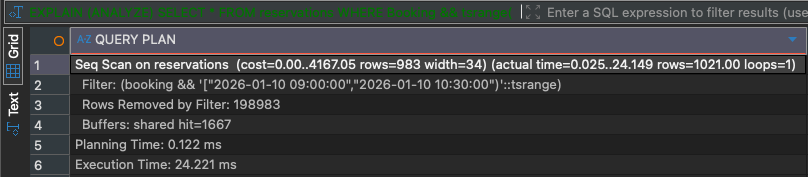
Let’s create now a GiST index to improve that query:

-- Create a GiST Index
CREATE INDEX idx_Reservations_Booking
ON Reservations
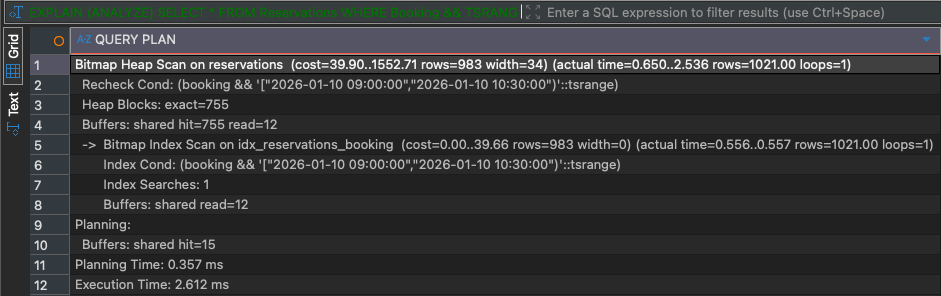
USING GIST (Booking);

When we rerun the query, the query planner chooses a Bitmap Index Scan operator (in combination with a Bitmap Heap Scan operator), and the query finishes in only 2 – 3ms:

SP-GiST in Practice: Prefix Searches on Text

While GiST is ideal for overlapping data, it becomes inefficient as soon as values belong to exactly one logical partition. In these cases, PostgreSQL does not need to manage overlapping regions or perform expensive rechecks. This is precisely the problem space where SP-GiST excels. SP-GiST stands for Space-Partitioned Generalized Search Tree. Unlike GiST, which allows index entries to overlap, SP-GiST divides the search space into non-overlapping regions. Each value belongs to exactly one partition, which allows PostgreSQL to navigate the index structure with very high precision.

Internally, SP-GiST is not a single data structure but a framework for several space-partitioning strategies. Common examples include tries for text prefixes, quadtrees for spatial points, and hierarchical trees for IP address ranges. The important aspect is not the specific structure, but the guarantee that partitions do not overlap. For SQL Server developers, this concept often feels familiar even if the name does not. Many performance optimizations in SQL Server attempt to create similar properties by carefully designing keys, prefixes, or computed columns. SP-GiST makes this approach explicit and native: the index itself understands how the data space is divided.

This makes SP-GiST particularly effective for prefix searches on text, point-based spatial data, and hierarchical values such as IP addresses. In these scenarios, the planner can traverse the index structure directly to the relevant partition, without scanning unrelated branches or performing overlap checks. The result is an index access path that is both fast and predictable, especially on large datasets with strong structural patterns. When data naturally forms a hierarchy rather than a range, SP-GiST is usually the most efficient indexing strategy PostgreSQL can offer.

Let’s have again a look on a concrete example. The following code creates a table, and inserts some test data into it:

-- Create a simple table
CREATE TABLE Users
(
    ID       BIGINT GENERATED ALWAYS AS IDENTITY PRIMARY KEY,
    Username TEXT
);

-- Insert some test data
INSERT INTO Users (Username) VALUES
('klaus'),
('klara'),
('karl'),
('kevin'),
('sarah'),
('stephan'),
('simon'),
('sebastian');

-- Additional test data to make the table larger
INSERT INTO users (username)
SELECT
    prefix || '_' || gs::text
FROM (
    SELECT
        CASE (random()*5)::int
            WHEN 0 THEN 'kla'
            WHEN 1 THEN 'kar'
            WHEN 2 THEN 'kev'
            WHEN 3 THEN 'sar'
            ELSE 'ste'
        END AS prefix
) p
CROSS JOIN generate_series(1, 200000) gs;

-- Update Statistics
ANALYZE Reservations;

When you run the following query without a SP-GiST index, PostgreSQL generates you a query plan with a Sequential Scan operator, that runs on my machine for around 16ms:

EXPLAIN (ANALYZE)
SELECT * FROM Users
WHERE Username LIKE 'kla%';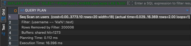

Let’s create now a SP-GiST index to improve that query:

-- Create a SP-GiST Index
CREATE INDEX idx_Users_Username
ON Users
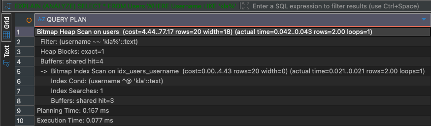
USING SPGIST (Username);

When we rerun the query, the query planner chooses again a Bitmap Index Scan operator, and the query finishes in less than a millisecond:

Final Thoughts: A Mental Shift for SQL Server Developers

The most important change when moving from SQL Server to PostgreSQL is not learning new syntax – it is learning a new way of thinking about indexes:

• SQL Server primarily optimizes for order
• PostgreSQL optimizes for meaning

GiST allows indexes to understand relationships like overlap, containment, and distance. SP-GiST allows indexes to exploit clean partitions in hierarchical or prefix-based data. Once you realize that operators like && are not just syntax sugar but index-aware semantic operations, the design starts to feel natural. PostgreSQL is not asking you how to express a condition efficiently – it is asking you to express what the condition means.

Thanks for your time,

-Klaus