You know the problem: the “Estimated Number of Rows” in an operator in the Execution Plan is 42, but you know that 42 isn’t the correct answer to this query. You have also heard some time ago that SQL Server uses statistics to make that estimation. But how can you interpret these statistics to understand from where the estimation is coming from?

Today I want to talk about statistics in SQL Server, and how SQL Server internally stores the estimation values in the so-called Histogram and the Density Vector.

Histogram

Let’s have a first look on the histogram. The idea behind the histogram is to store the data distribution of a column in a very efficient, compact way. Every time when you create an index on your table (Clustered/Non-Clustered Index), SQL Server also creates under the hood a statistics object for you. And this statistics object describes the data distribution in that specific column. Imagine you have an order table, and a column named Country. You have some sales in US, in the UK, in Austria, in Spain, and Switzerland. Therefore you can visualize the data distribution in that column like in the following picture.

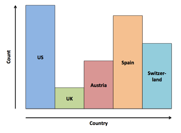
What you are seeing in that picture is a histogram – you are just describing the data distribution with some bars: the higher the bar is, the more records you have for that specific column value. And the same concept and format is used by SQL Server. Let’s have now a look on a more concrete example. In the AdventureWorks2012 database you have the table SalesOrderDetail and within that table you have the column ProductID. That column stores the ID of the product that was tight to that specific sale. In addition there is also an index defined on that column – means that SQL Server has also created a statistics object that describes the data distribution within that column.

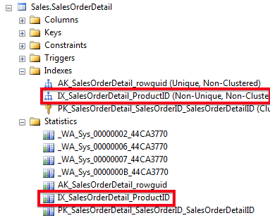
You can have a look into the statistics object by opening the properties window of it within SQL Server Management Studio, or you can use the command DBCC SHOW_STATISTICS to return the content of the statistics object in a tabular format:

-- Show the statistics for a given index
DBCC SHOW_STATISTICS ('Sales.SalesOrderDetail', IX_SalesOrderDetail_ProductID)
GO

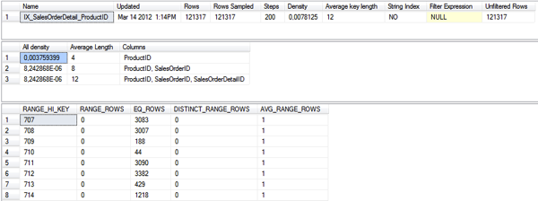
As you can see from the previous screen shot, the command returns you 3 different result sets:

• General information about the statistics object
• Density Vector
• Histogram

Within this blog posting we will concentrate on these 3 parts, and how they are used for the so-called Cardinality Estimation (the calculation of the estimated number of rows). Let’s run now a very simple query against the table SalesOrderDetail. As you can see from the following listing we are restricting for a specific ProductID:

-- SQL Server uses the EQ_ROWS to make the estimation, because the value is directly
-- available in the histogram.
-- 3083 are estimated for the the Filter operator
SELECT * FROM Sales.SalesOrderDetail
WHERE ProductID = 707
GO

The query itself returns 3.083 rows out from 121.317. Because we haven’t defined a Covering Non-Clustered Index (which isn’t here possible, because of the SELECT *), the query itself is over the Tipping Point, and you can see from the Execution Plan that SQL Server has chosen a Clustered Index Scan operator.

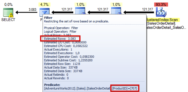
In the Execution Plan you can see at the end (or the beginning) a Filter operator, where SQL Server restricts the result set on the ProductID of 707. And the estimation is here 3.083 rows. It seems that we have here very accurate statistics. But the question is from where this estimation comes from. When you look at the histogram, you can see that we have multiple rows (up to 200 so-called Steps), which are describing the data distribution for the column ProductID. Every row in the histogram has the following columns:

• RANGE_HI_KEY
• RANGE_ROWS
• EQ_ROWS
• DISTINCT_RANGE_ROWS
• AVG_RANGE_ROWS

As you can see from the column RANGE_HI_KEY, there are 3083 records with the ProductID 707. This means that we have for that specific ProductID an exact match in the histogram. In that case SQL Server is using the value from the column EQ_ROWS (Equality Rows) to produce the result of the Cardinality Estimation – in our case 3.083 rows. That’s the estimation that you can see in the Filter operator in the Execution Plan.

Let’s have a look on the following query.

-- The value "915" isn't available directly in the histogram, therefore SQL Server uses
-- the AVG_RANGE_ROWS to make the estimation.
-- There are 150 records between the values 910 and 916 with 4 distinct values (DISTINCT_RANGE_ROWS).
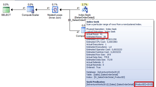
-- Therefore SQL Server estimates 150/4 = 37,5 rows for the Non-Clustered Index Seek.
SELECT * FROM Sales.SalesOrderDetail
WHERE ProductID = 915
GO

Here we are restricting on the ProductID of 915. But when you look into the histogram, you can see that there is no value for that specific ProductID. The histogram stores the values 910 and 916, and we have a gap between both values. This gap consists of 150 rows (RANGE_ROWS), excluding the values 910 and 916. And within these 150 rows we have 4 distinct values (DISTINCT_RANGE_ROWS). This means that our selectivity for a value between 910 and 916 is 37,5 (AVG_RANGE_ROWS = 150 / 4).

So in that case SQL Server estimates for the value 915 37,5 rows as you can see from the Execution Plan. In reality the Non-Clustered Index Seek operator returns 41 rows. Not a bad estimation.

As you can see from this example, SQL Server is also able to calculate a Cardinality Estimation when you have a non exact match in the histogram. For this reason you have the columns RANGE_ROWS and DISTINCT_RANGE_ROWS in the histogram. The histogram itself isn’t very hard to understand as you can see from this explanation. One very important thing about the histogram is the fact that SQL Server generates you the histogram only for the first index key column that is part of your index. For all subsequent index key columns SQL Server only stores the selectivity of the column in the Density Vector. Therefore you should always make sure that the column with the highest selectivity is the first one in your composite index key.

Density Vector

Let’s have a look on this mysterious density vector. When you have a look on the Non-Clustered Index IX_SalesOrderDetail_ProductID, the index is only defined on the column ProductID. But in every Non-Clustered Index SQL Server also has to stored the Clustered Key at least as a logical pointer in the leaf level of the index. When you have defined a Non-Unique Non-Clustered Index, the Clustered Key is also part of the navigation structure of the Non-Clustered Index. The Clustered Key on table SalesOrderDetail is a composite one, on the columns SalesOrderID and SalesOrderDetailID.

This means that our Non-Unique Non-Clustered Index consists in reality of the columns ProductID, SalesOrderID, and SalesOrderDetailID. Under the hoods you have a composite index key. This also means now that SQL Server has generated a density vector for the other columns, because only the first column (ProductID) is part of the histogram, that we have already seen in the earlier section. When you look at the output of the DBCC SHOW_STATISTICS command, the density vector is part of the second result set that is returned:

SQL Server stores here the selectivity, the density of the various column combinations.For example, we have an All Density Value for the column ProductID of 0,003759399. You can also calculate (and verify) this value at your own by dividing 1 by the number of distinct values in the column ProductID:

-- The "All Density" value for the column ProductID: 0,0037593984962406015
SELECT 1 / CAST(COUNT(DISTINCT ProductID) AS NUMERIC(18, 2)) FROM Sales.SalesOrderDetail
GO

The All Density Value for the column combinations ProductID, SalesOrderID and ProductID, SalesOrderID, SalesOrderDetailID is 8,242867858585359018109580685312e-6. You can again verify this, by dividing 1 by the number of distinct value in the columns ProductID, SalesOrderID, or ProductID, SalesOrderID, SalesOrderDetailID. In our case these values are unique (because they are part of the Clustered Key), so you calculate 1 / 121.317 = 8,242867858585359018109580685312e-6. The question is now, how SQL Server is using these density vector values for the cardinality estimation itself?

Let’s have a look on the following query:

-- SQL Server uses the reciprocal in a GROUP BY to make an estimation how
-- much rows are returned:
-- Estimation for the Stream Aggregate: 266
SELECT ProductID FROM Sales.SalesOrderDetail
GROUP BY ProductID
GO

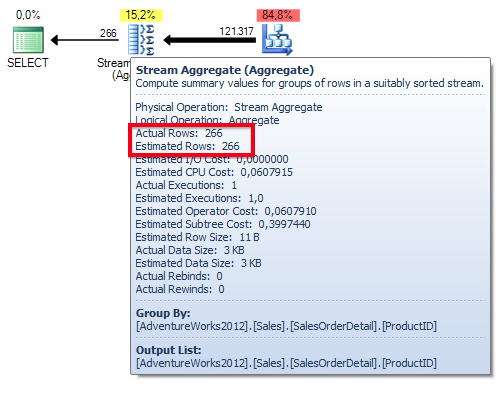
As you can see we are performing a GROUP BY on the column ProductID. In that case SQL Server is using the reciprocal of the density vector value of the column ProductID to estimate the number of rows for the Stream Aggregate operator: 1 / 0,0037593984962406015 = 266. When you have a look on the Execution Plan in the following picture, you can see the estimation of 266 rows for the Stream Aggregate operator.

When you are dealing with local variables in your T-SQL statements, SQL Server can’t sniff any parameter values anymore, and falls back to the density vector to perform the cardinality estimation. Let’s have a look on the following query.

-- SQL Server also uses the Density Vector when we are working with local variables
-- and equality predicates.
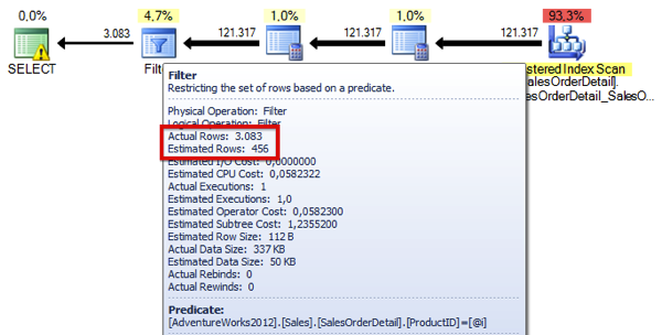
-- SQL Server estimates for the Non-Clustered Index Seek 456 records: 121317 * 0,003759 = 456
-- Every variable value gives us the same estimation.

-- Estimated: 456
-- Actual: 3083
DECLARE @i INT = 707

SELECT * FROM Sales.SalesOrderDetail
WHERE ProductID = @i

SQL Server estimates for the Filter operator 456 rows (121.317 * 0,0037593984962406015), and in reality we are returning only 44 rows.

When you are dealing with local variables in combination with inequality predicates, SQL Server isn’t using the density vector values anymore, and just assumes that 30% of the rows are returned.

-- When we are using an inequality predicate (">", "<") SQL Server assumes 30% for the
-- estimated number of rows.
-- Estimated: 36.395 (121.317/36.395 = 3,33)
-- Actual: 44
DECLARE @i INT = 719

SELECT * FROM Sales.SalesOrderDetail
WHERE ProductID > @i
GO

As you can see from the following Execution Plan, SQL Server always estimates 36.395 rows, because this is 30% of the rows from the table (121.317 * 0,30)

Summary

In this blog posting you have learned how SQL Server is using the underlying statistics objects to perform the cardinality estimation for our queries. As you have seen, a statistics object always has 2 very important parts: the histogram, and the density vector. Within the histogram SQL Server can estimate very easy, how many rows on average are returned for a specific query. Because the histogram is only created for the first column in a composite index key, SQL Server stores in addition in the density vector the selectivity of the other columns. And as you have seen these selectivity values are also used at various stages during the cardinality estimation.

If you are interested how you can draw an actual histogram with the GEOMETRY data type within SQL Server Management Studio, I highly recommend to check out Mark Wilkinson’s blog posting about it – really nice! 🙂

Thanks for reading

-Klaus